Animal model with GRM

This is a tutorial about how to fit an ‘animal model’ with GRM (genetic relationship matrix). We provide the sample with the Seychelles warbler data subset including body mass, tarsus length, and also other factors data of 36 individuals and the GRM were calculated from 10k snps genomic data filtered with PLINK -maf0.05 ).

dataset and GRM files can be downloaded from the Wamwiki github

Why do you want a GRM?

• NGS is (relatively) getting cheaper
• More information to estimate the relatedness, sometimes (like the warblers) the social pedigree can contain errors due to wrong observations or extra-pair paternity…
• No pedigree information in your study
• …

Before go to create a GRM, it is better to check the population structure by simply checking with a PCA plot. Or you can check the Fst of your dataset.

The method to generate GRM

Preparation - download and setup GCTA

There are many methods and tools (e.g., PLINK, NgsRelate* or R packages like ‘qgg’) to estimate the relatedness between individuals and generate a GRM, here is an example by using GCTA -grm flag. Note: NgsRelate accepts genotype likelihood input and vcf input

There is a flowchart to show the input file types for different methods to get a GRM

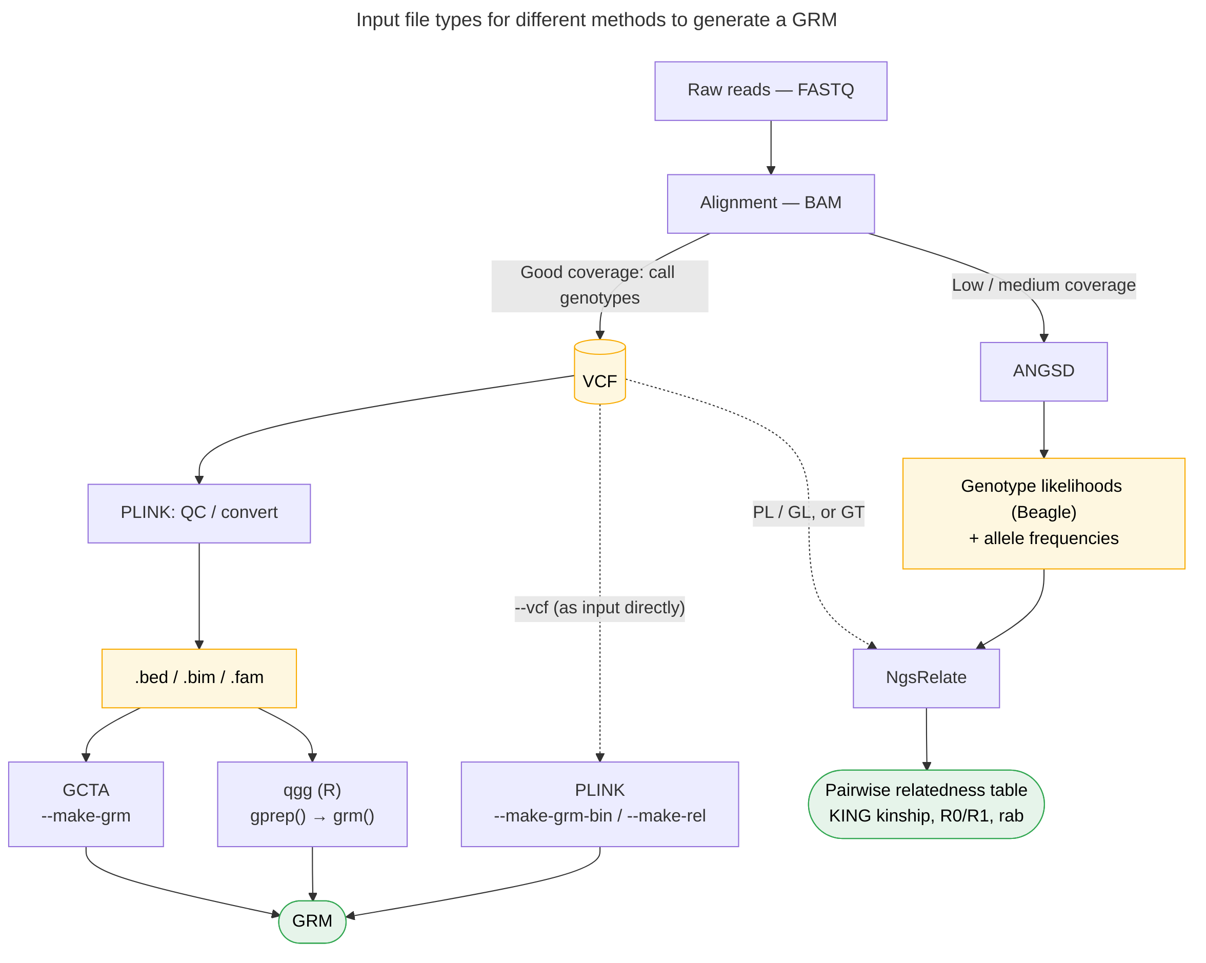
GCTA is a tool developed to study quantitative genetics based on genomic data, there is a function (–make-grm) which could estimate genetic relatedness from SNPs.

GCTA comes as a pre-compiled executable from the Yang Lab, You need to download the executable files on GCTA website, with builds for Linux, macOS, and Windows. Unzip it, inside the folder is the executable: gcta64 on Linux/Mac, gcta64.exe on Windows.

Here is the explanation of --make-grm function from GCTA website: Estimate the genetic relationship matrix (GRM) between pairs of individuals from a set of SNPs and save the lower triangle elements of the GRM to binary files.

For R (or the terminal) to find it when you just type gcta64, either add the folder containing it to your system ‘PATH’, or give the full path to the executable in your command (e.g. “/path/to/gcta64 –bfile …”). If you skip this, you’ll get a “command not found” error.

Laptop, workstation, or HPC?

For a relative small dataset (10k SNPs, ~1000 individuals) a personal laptop is completely fine, and this will finish in minutes. Here, we only have 36 individuals, this will complete in seconds.

But you need a workstation or HPC once you get into the 1,000 to 10,000 of individuals and 100,000 to 1,000,000 of SNPs, where the matrix becomes many gigabytes (that’s also when GCTA’s –make-grm-part chunking becomes useful). For this step in the tutorial, no special hardware is needed.

If you want to check the details of making a GRM with GCTA, you can check here.

# You could run GCTA in R by using system() function or run the command line in terminal

#system("/your/path/to/gcta64 or gcta64.exe --bfile filterd.final.autosome.maf0.05_bodymass_h2_gwas_50ind_10k_WAMBAM  --make-grm --autosome-num 29 --out filterd.final.autosome.maf0.05.36ind.10k.WAMBAM")

Notes:

–bfile your PLINK binary files, this isn’t one file but a trio that share the same prefix: a .bed file (the genotype calls in compact binary form), a .bim file (one row per SNP: chromosome, ID, position, alleles), and a .fam file (one row per individual: IDs, sex, phenotype). You supply only the shared prefix with no extension, and GCTA finds all three

–make-grm, compute the Genetic Relationship Matrix flag

–autosome-num 29, tells GCTA how many pairs of autosomes the species has. This matters because GCTA defaults to humans (22 autosomes), so for any non-human species you must set it explicitly or the autosome selection will be wrong. 29 indicates the seychelles warbler with 29 autosome pairs

–out prefix, the prefix for all output files. Everything GCTA writes here with the prefix you provided

There are 3 output files from GCTA: grm.bin, grm.id, grm.N.bin, you need to put them under the same directory

Model fitting

Here, we fit the data into animal model in brms

First, you need to install and load all the packages, you can check brms usage tutorial to know how to setup first

#install.packages(c("readr","genio","brms","cmdstanr","rstan"))
##setup your work directory
setwd("~/wamwiki.github.io/content/en/docs/Univariate/GRM/")
library(readr)
library(genio)
library(MASS)
library(brms)
library(cmdstanr)
library(tidybayes)
library(rstan)
library(dplyr)
library(ggplot2)

load the dataset, GRM

dataset <- read.csv("dataset_bodycondition_sw.csv")
grm.data <- genio::read_grm("filterd.final.autosome.maf0.05.36ind.10k.WAMBAM.grm")

## Reading: filterd.final.autosome.maf0.05.36ind.10k.WAMBAM.grm.id

## Reading: filterd.final.autosome.maf0.05.36ind.10k.WAMBAM.grm.bin

## Reading: filterd.final.autosome.maf0.05.36ind.10k.WAMBAM.grm.N.bin

#Check the number of SNPs used for GRM
#So there's some missing data (SNPs that didn't match in pairs) in the dataset, but not much to worry about. The counts range from 9,312 to 9,970 SNPs per pair, meaning every relatedness estimate is built on at least ~9,300 markers.

summary(grm.data$M[lower.tri(grm.data$M)])

##    Min. 1st Qu.  Median    Mean 3rd Qu.    Max. 
##    9312    9769    9852    9809    9894    9947

#Matrix::nearPD() finds the nearest positive-definite matrix to the one you give it. animal models use the GRM as a covariance matrix, which must be positive definite to be both statistically valid and computationally usable, the model equations require inverting and factoring the matrix, which fails if it's singular or has negative eigenvalues
#It is not always necessary to force positive definite your GRM, nearPD() is the safety net that guarantees the matrix satisfies that requirement
GRM_pd <- as.matrix(Matrix::nearPD(grm.data$kinship)$mat)

# You can check your GRM before positive definite step
# Smallest eigenvalue of the raw GRM: > 0 means already positive definite, then you can use your raw GRM
min(eigen(grm.data$kinship, symmetric = TRUE, only.values = TRUE)$values)

## [1] -0.009069228

Check if the dataset and GRM with the same individual

dataset_birds <- unique(dataset$BirdID)
cat("Birds in dataset:", length(dataset_birds), "\n")

## Birds in dataset: 36

cat("Birds in GRM:", nrow(GRM_pd), "\n")

## Birds in GRM: 36

cat("Overlap:", sum(dataset_birds %in% rownames(GRM_pd)), "\n")

## Overlap: 36

cat("Missing from GRM:", sum(!dataset_birds %in% rownames(GRM_pd)), "\n")

## Missing from GRM: 0

cat("Missing from model:", sum(!rownames(GRM_pd) %in% dataset_birds), "\n")

## Missing from model: 0

Keep only birds present in model and GRM

birds_in_both <- dataset_birds[dataset_birds %in% rownames(GRM_pd)]
cat("Birds to use in GRM animal model:", length(birds_in_both), "\n")

## Birds to use in GRM animal model: 36

GRM_sub <- GRM_pd[as.character(birds_in_both), as.character(birds_in_both)]

dim(GRM_sub)

## [1] 36 36

data_final <- dataset[dataset$BirdID %in% birds_in_both, ]

Be careful with the prior, but in general the default prior works well. Here we used the default prior get from get_prior() function.

# get priors from get_prior() function
my_priors <- c(prior(normal(0, 1),class = b,coef = age_year),
               prior(normal(0, 0.5),class = b,coef = Iage_yearE2), 
               prior(normal(0, 2),class = b,coef = RightTarsus), 
               prior(normal(0, 1),class = b,coef = SexEstimate),  
               prior(normal(0, 1),class = b,coef = summer),
               prior(normal(0, 1),class = b,coef = minutes_s),
               prior(normal(0, 1),class = b,coef = avg_invert),
               prior(normal(0, 1),class = b,coef = group_size),
               # fixed effects priors were provided above
               prior(normal(15.5, 3),class = Intercept), # intercept prior
               prior(student_t(3, 0, 1), class = sd), # random effect sd priors
               prior(student_t(3, 0, 1), class = sigma)) # residual sd prior

We set chains = 4 to let the model to run 4 MCMC chains at the same time, and also saved as rda file, brms model structure:

model_grm <- brm(
  BodyMass ~ age_year + I(age_year^2) + RightTarsus + SexEstimate + summer +minutes_s + avg_invert + group_size + (1 | gr(animal, cov = GRM_pd)) + (1 | BirdID) + (1 | BirthYear) + (1 | CatchYear) + (1 | Observer),
  data    = data_final,
  data2   = list(GRM_pd = GRM_pd),
  family  = gaussian(),
  prior   = my_priors,
  warmup  = 1500,
  iter    = 11500,
  chains  = 4,
  cores   = 4,
  seed    = 123,
  file    = "m_brms_GRM",
  backend = "cmdstanr")

check the ESS, Rhat and check_hmc_diagnostics() to evaluate the animal model:

summary(model_grm)

##  Family: gaussian 
##   Links: mu = identity; sigma = identity 
## Formula: BodyMass ~ age_year + I(age_year^2) + RightTarsus + SexEstimate + summer + minutes_s + avg_invert + group_size + (1 | gr(animal, cov = GRM_pd)) + (1 | BirdID) + (1 | BirthYear) + (1 | CatchYear) + (1 | Observer) 
##    Data: data_final (Number of observations: 87) 
##   Draws: 4 chains, each with iter = 11500; warmup = 1500; thin = 1;
##          total post-warmup draws = 40000
## 
## Multilevel Hyperparameters:
## ~animal (Number of levels: 36) 
##               Estimate Est.Error l-95% CI u-95% CI Rhat Bulk_ESS Tail_ESS
## sd(Intercept)     0.51      0.24     0.04     0.93 1.00     6405    12625
## 
## ~BirdID (Number of levels: 36) 
##               Estimate Est.Error l-95% CI u-95% CI Rhat Bulk_ESS Tail_ESS
## sd(Intercept)     0.39      0.24     0.02     0.85 1.00     5986    15672
## 
## ~BirthYear (Number of levels: 20) 
##               Estimate Est.Error l-95% CI u-95% CI Rhat Bulk_ESS Tail_ESS
## sd(Intercept)     0.20      0.16     0.01     0.58 1.00    17353    21427
## 
## ~CatchYear (Number of levels: 20) 
##               Estimate Est.Error l-95% CI u-95% CI Rhat Bulk_ESS Tail_ESS
## sd(Intercept)     0.15      0.12     0.01     0.44 1.00    18561    24015
## 
## ~Observer (Number of levels: 25) 
##               Estimate Est.Error l-95% CI u-95% CI Rhat Bulk_ESS Tail_ESS
## sd(Intercept)     0.21      0.16     0.01     0.59 1.00    11747    20612
## 
## Regression Coefficients:
##             Estimate Est.Error l-95% CI u-95% CI Rhat Bulk_ESS Tail_ESS
## Intercept      18.86      3.96    11.07    26.60 1.00    46982    30615
## age_year        0.11      0.09    -0.07     0.29 1.00    42264    30117
## Iage_yearE2    -0.01      0.01    -0.02     0.01 1.00    37350    29728
## RightTarsus    -0.15      0.16    -0.46     0.17 1.00    48268    30677
## SexEstimate     1.80      0.36     1.08     2.50 1.00    46365    29003
## summer         -0.01      0.21    -0.41     0.40 1.00    63408    32598
## minutes_s       0.15      0.11    -0.06     0.35 1.00    40911    31233
## avg_invert     -0.04      0.07    -0.17     0.10 1.00    56743    30688
## group_size     -0.19      0.08    -0.36    -0.03 1.00    37239    31108
## 
## Further Distributional Parameters:
##       Estimate Est.Error l-95% CI u-95% CI Rhat Bulk_ESS Tail_ESS
## sigma     0.61      0.08     0.47     0.77 1.00    11485    21178
## 
## Draws were sampled using sample(hmc). For each parameter, Bulk_ESS
## and Tail_ESS are effective sample size measures, and Rhat is the potential
## scale reduction factor on split chains (at convergence, Rhat = 1).

rstan::check_hmc_diagnostics(model_grm$fit)

## 
## Divergences:

## 0 of 40000 iterations ended with a divergence.

## 
## Tree depth:

## 0 of 40000 iterations saturated the maximum tree depth of 10.

## 
## Energy:

## E-BFMI indicated no pathological behavior.

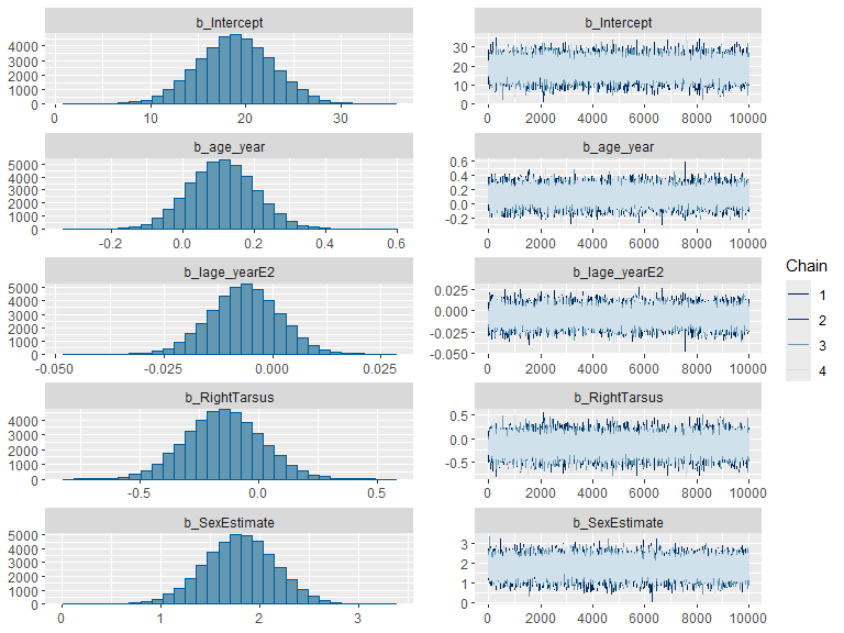
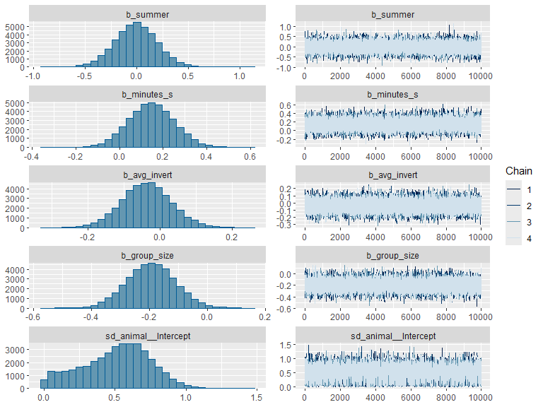
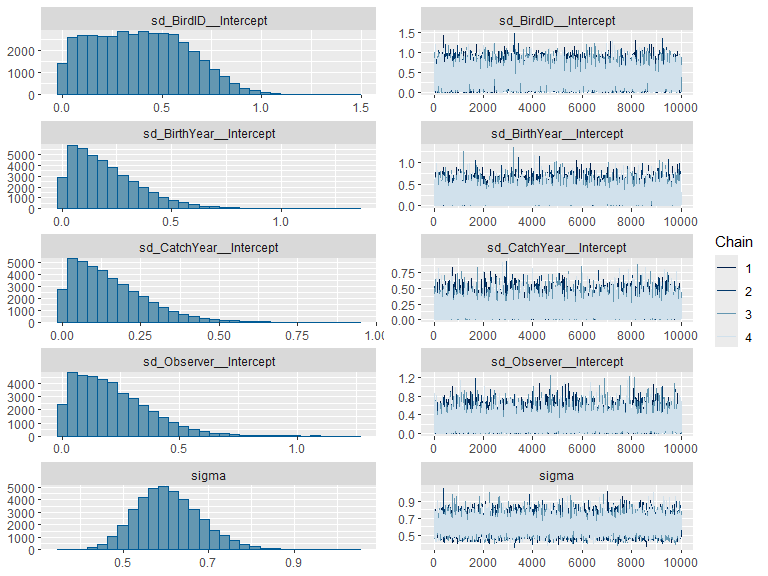
Also check the mcmc traces if they mixed well:

plot(model_grm)

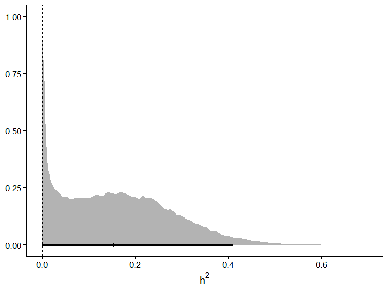
The heritability (h2) can be computed:

#Vf (fixed effect variance) calculation
mu_fixed <- posterior_linpred(model_grm, re_formula = NA)
# variance per posterior draw
Vf_GRM <- apply(mu_fixed, 1, var)

h2_draws_Vf_GRM <- model_grm %>%
  spread_draws(sd_animal__Intercept, sd_BirdID__Intercept, sd_BirthYear__Intercept,
               sd_CatchYear__Intercept, sd_Observer__Intercept, sigma) %>%
  mutate(Vf  = Vf_GRM,
         Vg  = sd_animal__Intercept^2,
         Vpe = sd_BirdID__Intercept^2,
         Vby = sd_BirthYear__Intercept^2,
         Vcy = sd_CatchYear__Intercept^2,
         Vobs= sd_Observer__Intercept^2,
         Ve  = sigma^2,
         Vp  = Vg + Vpe + Vby + Vcy + Vobs + Ve + Vf,
         h2  = Vg / Vp,
         repeatability = (Vg + Vpe) / Vp,
         CVa = 100 * (sd_animal__Intercept / mean(data_final$BodyMass, na.rm = TRUE)))

We can also get the point estimation:

h2_draws_Vf_GRM %>% mean_hdi(h2)

## # A tibble: 2 × 6
##      h2       .lower .upper .width .point .interval
##   <dbl>        <dbl>  <dbl>  <dbl> <chr>  <chr>    
## 1 0.161 0.0000000211  0.361   0.95 mean   hdi      
## 2 0.161 0.366         0.371   0.95 mean   hdi

h2_draws_Vf_GRM %>% mean_hdi(repeatability)

## # A tibble: 1 × 6
##   repeatability .lower .upper .width .point .interval
##           <dbl>  <dbl>  <dbl>  <dbl> <chr>  <chr>    
## 1         0.267 0.0822  0.459   0.95 mean   hdi

h2_draws_Vf_GRM %>% mean_hdi(CVa)

## # A tibble: 1 × 6
##     CVa  .lower .upper .width .point .interval
##   <dbl>   <dbl>  <dbl>  <dbl> <chr>  <chr>    
## 1  3.25 0.00896   5.58   0.95 mean   hdi

Plot the h2

ggplot(h2_draws_Vf_GRM, aes(x = h2)) +
  stat_halfeye(.width = c(0.95), fill = "grey70", color = "black") +
  geom_vline(xintercept = 0, linetype = "dashed", linewidth = 0.4) +
  scale_x_continuous(limits = c(0, NA)) +
  labs(x = expression(h^2), y = NULL) +
  theme_classic(base_size = 16)